STAT 5010 - An example survey

study	p_1	p_2	q_1	q_2	n
1	0.4830	0.3920	0.4610	0.4160	2046
2	0.4100	0.3500	0.4200	0.3600	1149
3	0.4660	0.3310	0.4650	0.3490	1112
4	0.4601	0.3222	0.4082	0.3586	1112
5	0.4400	0.3200	0.3970	0.3300	1082
6	0.3880	0.2930	0.3820	0.3060	1484

study	DiP	se	CI.lower	CI.upper
1	2.18	1.54	-0.83	5.23
2	-0.97	2.05	-4.96	3.05
3	0.11	2.12	-4.05	4.23
4	5.14	2.09	0.99	9.26
5	4.30	2.14	0.09	8.50
6	0.63	1.79	-2.90	4.11

study	DiD	se	CI.lower	CI.upper
1	4.57	2.88	-1.03	10.22
2	0.05	3.63	-6.96	7.14
3	1.89	3.78	-5.58	9.35
4	8.74	3.69	1.44	15.92
5	5.29	3.70	-1.85	12.66
6	1.95	3.03	-4.04	7.88

Joint distribution of the two questions

Apparently, the responses to the two question are correlated.
However we only the marginal distributions for each question.
We need to model the joint distribution directly.
Let Q1 be the first question (A vs B) and Q2 be the second question (A’ vs B).
Suppose the joint distribution is

Q1\Q2 A’ B no response

A $ρ_{1}$ $ρ_{12}$ $γ$

B $ρ_{21}$ $ρ_{2}$ $γ$

no response $γ$ $γ$ $ρ_{3}$
The parameter is $θ = (ρ_{1}, ρ_{2}, ρ_{3}, ρ_{12}, ρ_{21}, γ)$ , where $ρ_{1} + ρ_{2} + ρ_{3} + ρ_{12} + ρ_{21} + 4 γ = 1$ .
Denote the counts by $n_{i j}$ , where $i, j \in {1, 2, 3} = {A, B, no response}$ .

Q1\Q2	A’	B	no response
A	$ρ_{1}$	$ρ_{12}$	$γ$
B	$ρ_{21}$	$ρ_{2}$	$γ$
no response	$γ$	$γ$	$ρ_{3}$

Interpretation of the parameters

$ρ_{1}$ : the proportion of people that always prefer A type.
$ρ_{2}$ : the proportion of people that always prefer B type.
$ρ_{3}$ : the proportion of people that always give no response.
$ρ_{12}$ : the proportion of people that prefer $A > B > A^{'}$ .
$ρ_{21}$ : the proportion of people that prefer $A^{'} > B > A$ .
$γ$ : the proportion of people that answer only one of the two questions.

Missing Data

We have observed $Y = [n_{1 \cdot}, n_{2 \cdot}, n_{3 \cdot}, n_{\cdot 1}, n_{\cdot 2}]^{T}$ , where $n_{i \cdot} = \sum_{j} n_{i j}$ and $n_{\cdot j} = \sum_{i} n_{i j}$ .
Let $U = [n_{11}, n_{12}, n_{13}, n_{21}, n_{22}, n_{23}, n_{31}, n_{32}, n_{33}]^{T}$ be the complete data.
If we also observe $Z = [n_{11}, n_{12}, n_{21}, n_{32}]^{T}$ , then $U$ can be recovered from $Y$ and $Z$ .
$Z$ is called the missing data.
Let $M$ be a matrix such that $U = M [\begin{matrix} Y \\ Z \end{matrix}] .$
The distribution of $U$ multinomial with parameter $(ρ_{1}, ρ_{12}, γ, ρ_{21}, ρ_{2}, γ, γ, γ, ρ_{3})$ .

Intuition

If we observe $U$ , we can find the posterior $π (θ ∣ U)$ .
Observing $U$ is equivalent to observing $Y$ and $Z$ and hence the posterior can be written as $π (θ ∣ Y, Z)$ .
However, $Z$ is missing, so we can not condition on $Z$ .
The most we can do is $π (θ, Z ∣ Y)$ .
By Bayes Theorem, $π (θ, Z ∣ Y) = \frac{p (Y, Z ∣ θ) π (θ)}{p (Y)} .$
The distribution $p (Y, Z ∣ θ)$ is available since $[Y^{T}, Z^{T}]^{T} = M^{- 1} U$ and $U$ is multinomial.
We can also consider the marginal posterior $π (θ ∣ Y) = \sum_{Z} π (θ, Z ∣ Y)$ .

Data (Survey 1)

Q1\Q2	A’	B	No response	Total
A	$437$	$409$	$120$	988
B	$358$	$327$	$99$	802
No response	$127$	$96$	$27$	256
Total	943	851	$252$	$2046$

The numbers in black are observed.
The numbers in red are my random guesses.
The numbers in blue are redundant as they can be computed from the others.

Sampling Algorithm

We need to sample from $π (θ, Z ∣ Y)$ .
The sampling is achieved by Gibbs sampler:
- sample $Z$ from $π (Z ∣ θ, Y)$
- sample $θ$ from $π (θ ∣ Z, Y)$ .
In our case, $π (Z ∣ θ, Y)$ is independent of $θ$ and the full conditionals $π (z_{i} ∣ z_{- i}, Y)$ are hypergeometric distributions.
You fill find that the derivation is the same as Fisher’s exact test.
The distribution $π (θ ∣ Z, Y)$ is exactly $π (θ ∣ U)$ , i.e., the posterior given the complete data.

Prior and posterior

We need to specify a prior for $θ = (ρ_{1}, ρ_{2}, ρ_{3}, ρ_{12}, ρ_{21}, 4 γ)$ .
For convenience, we choose $(ρ_{1}, ρ_{2}, ρ_{3}, ρ_{12}, ρ_{21}, 4 γ) \sim Dir (α_{1}, \dots, α_{6})$ .
The posterior given the complete data is $\begin{matrix} (ρ_{1}, ρ_{2}, ρ_{3}, ρ_{12}, ρ_{21}, 4 γ) ∣ U \sim Dir (α_{1} + n_{11}, α_{2} + n_{22}, α_{3} + n_{33}, α_{4} + n_{12}, \\ α_{5} + n_{21}, α_{6} + n_{13} + n_{23} + n_{31} + n_{32}) . \end{matrix}$

Analysis for Survey 1

source("../dataset/survey/survey_Missing.R")

Y <- c(988, 802, 256, 943, 851)
theta_sample <- single_survey_sampler(3000, Y)

	Q_2.A'	Q_2.B	Q_2.No response	total
Q_1.A	22.23	20.07	5.43	47.73
Q_1.B	18.09	16.30	5.43	39.82
Q_1.No response	5.43	5.43	1.59	12.45
total	45.75	41.80	12.45	100.00

Analysis for Survey 2

Y <- c(471, 402, 276, 483, 414)
theta_sample <- single_survey_sampler(3000, Y)

	Q_2.A'	Q_2.B	Q_2.No response	total
Q_1.A	17.19	14.81	8.83	40.83
Q_1.B	14.75	12.58	8.83	36.17
Q_1.No response	8.83	8.83	5.33	23.00
total	40.77	36.23	23.00	100.00

Meta analysis

We can also perform meta analysis by combining the 6 surveys.
Let $U_{i}$ be the complete data for survey $i$ .
A simple hierarchical model is $\begin{aligned} U_{i} ∣ θ_{i} & \overset{i n d}{\sim} Multinomial (θ_{i}), \\ θ_{i} ∣ α, ν & \overset{i i d}{\sim} Dir (α ν), \\ ν & \sim Dir (1, 1, 1, 1, 1, 1), \\ α & \sim Exp (0.001) \end{aligned}$
The complete data $U_{i}$ is obtained by generating the missing data $Z_{i}$ from $π (Z_{i} ∣ Y_{i})$ and then combining with the observed data $Y_{i}$ .
I wrote a function multi_survey_sampler to perform the meta analysis.

What is the question?

Suppose you have obtained posterior samples of $θ_{i} = (ρ_{1, i}, ρ_{2, i}, ρ_{3, i}, ρ_{12, i}, ρ_{21, i}, γ_{i})$ for $i = 1, \dots, 6$ .
What do you want to know?
Probably, you want to compare $ρ_{12, i}$ and $ρ_{21, i}$ for each $i = 1, \dots, 6$ .
You have several choices:
- use $η_{1, i} = ρ_{12, i} - ρ_{21, i} \in [- 1, 1]$ ;
- use $η_{2, i} = \log \frac{ρ_{12, i}}{ρ_{21, i}} \in (- \infty, \infty)$ ;
Since we are using the joint distribution, it is okay to subtract probabilities (although it is not recommended).
You cannot arbitrarily subtract conditional probabilities or marginal probabilities.
For example, it is meaningless to compute $\begin{aligned} P (X = 1) - P (Y = 0) or \\ P (X = 1 ∣ Y = 1) - P (X = 1 ∣ Y = 0) . \end{aligned}$

Analysis

source("../dataset/survey/survey_Missing.R")
survey_data <- read.csv("../dataset/survey/survey_data.csv",header = TRUE)
attach(survey_data)
N1 <- cbind(round(n*p_1), round(n*p_2))
N1 <- cbind(N1, n - N1[,1] - N1[,2])
N2 <- cbind(round(n*q_1), round(n*q_2))
N2 <- cbind(N2, n - N2[,1] - N2[,2])
detach(survey_data)
Y <- cbind(N1, N2[,1:2])
Y |> `colnames<-`(c("n_1.", "n_2.", "n_3.", "n_.1", "n_.2")) |> kable()

n_1.	n_2.	n_3.	n_.1	n_.2
988	802	256	943	851
471	402	276	483	414
518	368	226	517	388
512	358	242	454	399
476	346	260	430	357
576	435	473	567	454

Analysis

model <- stan_model("../dataset/survey/multi_survey.stan")
samples <- multi_survey_sampler(Y, model)

eta1 <- samples$theta[,4,] - samples$theta[,5,]
eta2 <- log(samples$theta[,4,]) - log(samples$theta[,5,])
eta1_overall <- samples$nu[,4] - samples$nu[,5]
eta2_overall <- log(samples$nu[,4]) - log(samples$nu[,5])

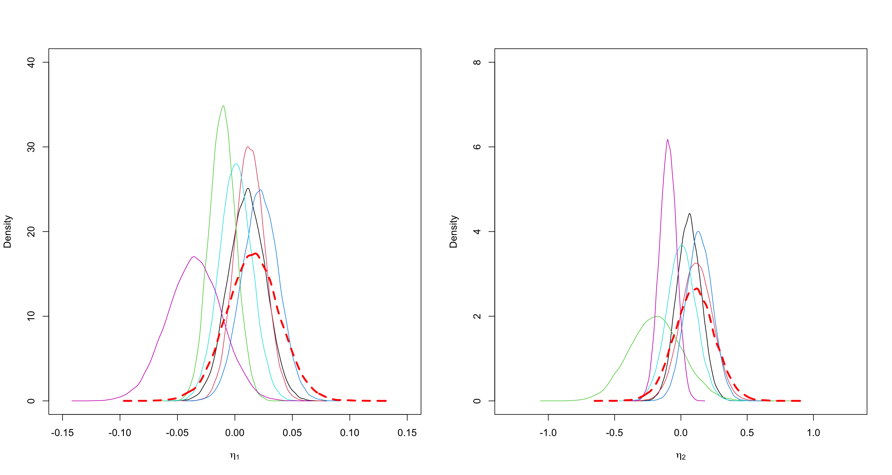
Results

$η_{1} = ρ_{12} - ρ_{21} =$ (prefer A > B > A’) - (prefer A’ > B > A)
$η_{2} = \log \frac{ρ_{12}}{ρ_{21}} =$ log(prefer A > B > A’) - log(prefer A’ > B > A)
The red dashed line is the overall estimate.

An example survey

An example survey

Survey Results

Assumptions

Parametric Bootstrap

Difference in Proportions

Difference in Differences

Bayesian Analysis

Joint distribution of the two questions

Interpretation of the parameters

Missing Data

Intuition

Data (Survey 1)

Sampling Algorithm

Prior and posterior

Analysis for Survey 1

Analysis for Survey 2

Meta analysis

What is the question?

Analysis

Analysis

Results

n_1.	n_2.	n_3.	n_.1	n_.2
988	802	256	943	851
471	402	276	483	414
518	368	226	517	388
512	358	242	454	399
476	346	260	430	357
576	435	473	567	454

n_1.	n_2.	n_3.	n_.1	n_.2
988	802	256	943	851
471	402	276	483	414
518	368	226	517	388
512	358	242	454	399
476	346	260	430	357
576	435	473	567	454

n_1.	n_2.	n_3.	n_.1	n_.2
988	802	256	943	851
471	402	276	483	414
518	368	226	517	388
512	358	242	454	399
476	346	260	430	357
576	435	473	567	454